We'll start our blogging journey with the first thing we all learn in our modelling career: Linear Regression. We will, however, add a fun twist to keep things interesting. Let us first recall the Linear Regression matrix definition:
\[ \boldsymbol{Y} = \boldsymbol{X \beta} + \boldsymbol{U} \]The notation is a bit weird as we denote the error matrix with $\boldsymbol{U}$, just bear with me, it will make more sense in the future. The idea is to approximate $\boldsymbol{Y}$ via matrix multiplication of $\boldsymbol{X}$ and $\boldsymbol{\beta}$ and minimizing the norm of the error matrix $\boldsymbol{U}$. This is probably the most studied statistical model in history and has a huge list of known problems and issues deriving mainly from the strict assumptions made when building the model. We will focus on a small detail concerning the optimization framework used in this naive Linear Regression.
Let me paint you a story: it's 2021 and I'm writing my master's thesis (This is the link for the curious). I'm trying to create a full mapping (and called it Label Adaptation) between 4 different credit rating agencies to fill in the missing points in my database. That is, I want to be able to approximate what agency A would have rated a given company if any of the other agencies have issued a rating for that same company. I constructed the algorithm to take into account all the different missing point combinations (just agency A is missing, both A and B are missing, both A and C and so on and so forth). I built the links by training a Linear Regression model using Ordinary Least Squares (OLS) as my optimization function for each combination and got the following results:
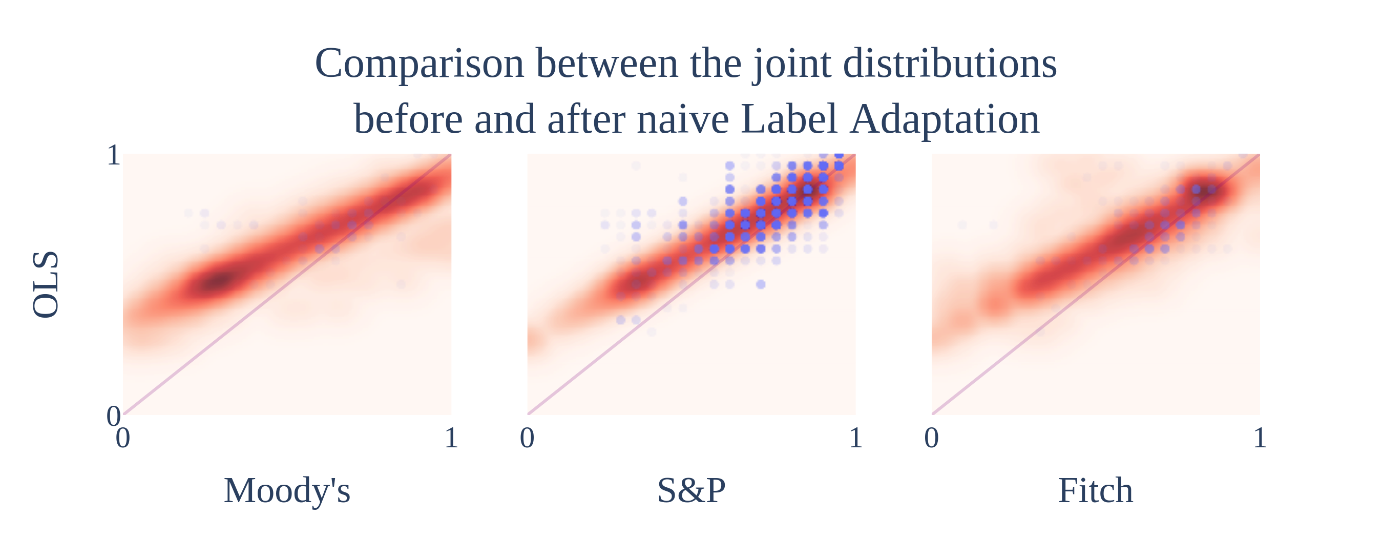
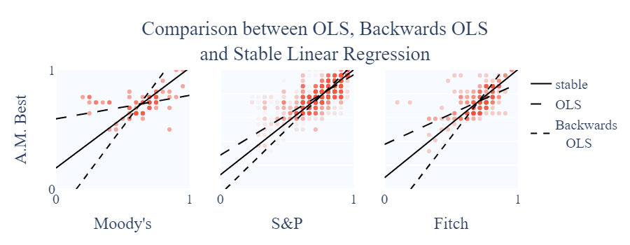
The $y$ axis contains the ratings given by A.M. Best (along with the regression fit) and the $x$ axis contains all the other agencies. This particular setup was done because A.M. Best is the smallest and most specialized of all the 4 agencies, with its focus being on insurance-related companies. I modified the domain of the ratings to homologate them, giving 0 to the worst possible rating and 1 to the best and then partitioning the range into equal parts depending on the number of different grades for each agency. The blue dots are the observed ratings and the heatmap are the predicted ratings using OLS and the mapping.
I could not help but notice that the OLS predicted A.M. best would over-rate companies that all other agencies would generally associate with low ratings (left side of the plots). After closer inspection, it seemed like the outliers in this section were skewing the OLS upwards, resulting in this weird artefact. I also figured I could fix it by adding another feature I wanted my mapping to have: stability.
What I mean by stability, in this context, is that the model for mapping agency $A$ to agency $B$ is homologous to the model for mapping agency $B$ to agency $A$. To check that outliers were indeed messing with this stability, I performed the forwards (predicting $\boldsymbol{Y}$ using $\boldsymbol{X}$) and backwards (predicting $\boldsymbol{X}$ using $\boldsymbol{Y}$) regression on A.M. Best against the other agencies. Then I modified the backwards regressions so that $\boldsymbol{Y}$ was left alone on one side of the equation, which should result in very close slope parameters. This, however, did not hold as seen in the next table.
| Intercept | Coefficient | |||
|---|---|---|---|---|
| Forward OLS | Backward OLS | Forward OLS | Backward OLS | |
| Moody's | 0.5895 | -0.2282 | 0.1967 | 1.4976 |
| S&P | 0.2846 | -0.0439 | 0.6757 | 1.0964 |
| Fitch | 0.3750 | -0.2852 | 0.5117 | 1.4488 |
Ok, both intercept and slope coefficients were way off considering my $[0, 1]$ range. I then created an extension on Linear Regression to account for stability as follows:
Definition. A linear regression problem is said to be stable given
if and only if $\boldsymbol{\beta} = \boldsymbol{\Gamma}^+$, with $\boldsymbol{\Gamma}^+$ is the pseudo inverse of $\boldsymbol{\Gamma}$.
Remark. The matrices $\boldsymbol{X} \in \mathbb{R}^{m \times (k + 1)}$, $\boldsymbol{Y} \in \mathbb{R}^{m \times (n + 1)}$ most of the time will be assumed to be of the form $\begin{bmatrix} 1 & \boldsymbol{x}_1 & \cdots & \boldsymbol{x}_k \end{bmatrix}$ and $\begin{bmatrix} 1 & \boldsymbol{y}_1 & \cdots & \boldsymbol{y}_n \end{bmatrix}$ respectively.
Correspondingly, $\boldsymbol{\beta} \in \mathbb{R}^{(k + 1) \times (n + 1)}$, $\Gamma \in \mathbb{R}^{(n + 1) \times (k + 1)}$ take the forms
I basically forced the parameter matrices to be homologous, and then modified the optimization functions to take into account both the $\boldsymbol{X}$ and $\boldsymbol{Y}$ errors (as previously only the $\boldsymbol{Y}$ errors were considered). I did not find an algebraic solution to the optimization function, as I was running low on time to turn the thesis in. However, I was able to avoid the issue by using numeric methods (namely Particle Swarm Optimization) to minimize this new error with almost no computational overhead. The trick was to use the bisection of the forward and backward regression as an initial guess, which after some testing appeared to always lay close to the final result.
The new model, on the individual tests, seems to be doing what it was designed to do. It is way more robust to outliers, and the forward and backward versions are homologous by definition. Now it was time to test it on the whole mapping to see if the original artefact was fixed.
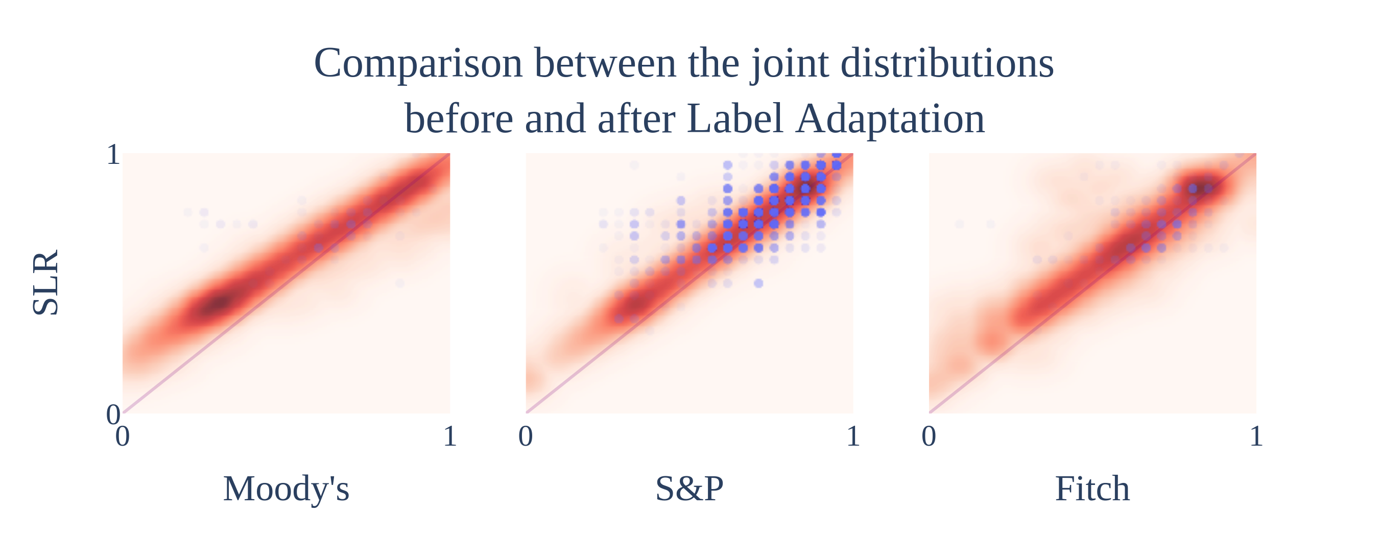
Success! The mapping + Stable Linear Regression combo works way better than the original setup. The next step would be to gather several other variables to help with the rating prediction, but that is a story for another day.